A detector hands you dots each frame. When a car slips behind a truck the dot vanishes, but the planner still needs the same car, in a smooth place, with the same id.
This notebook builds a tiny tracker that keeps ids on the right cars, then walks through the failure modes that break naive matching. The swap is the lesson.
Each idea shows up three times: a picture, a handful of numbers, then a few lines of code. Predict first, then run the cell. The paragraph after the cell says what was surprising, and what it would mean for a car.
import os, subprocess, sys
from pathlib import Path

import matplotlib
import matplotlib.pyplot as plt
import numpy as np

def keep_inline():
    matplotlib.use("module://matplotlib_inline.backend_inline", force=True)
    ip = None
    try:
        from IPython import get_ipython
        ip = get_ipython()
    except Exception:
        ip = None
    if ip is not None:
        ip.run_line_magic("matplotlib", "inline")

%matplotlib inline

def find_repo(start: Path) -> Path:
    for p in [start, *start.parents]:
        if (p / "modules" / "05_vector_space" / "kalman_tracker.py").is_file():
            return p.resolve()
    return start.resolve()

REPO = find_repo(Path.cwd())
if not (REPO / "modules" / "05_vector_space" / "kalman_tracker.py").is_file():
    dest = Path.cwd() / "self-driving-ai-course"
    if not (dest / "modules" / "05_vector_space" / "kalman_tracker.py").is_file():
        subprocess.run(
            ["git", "clone", "--depth", "1", "https://github.com/vvknyn/self-driving-ai-course.git", str(dest)],
            check=True,
        )
    REPO = dest.resolve()
os.chdir(REPO)

try:
    import scipy  # noqa: F401
except ImportError:
    subprocess.run([sys.executable, "-m", "pip", "install", "-q", "scipy"], check=True)
try:
    import pytest  # noqa: F401
except ImportError:
    subprocess.run([sys.executable, "-m", "pip", "install", "-q", "pytest"], check=True)

sys.path.insert(0, str(REPO / "modules" / "05_vector_space"))
from kalman_tracker import KalmanBoxTracker, MultiObjectTracker
from vector_lanes import VectorLane
from scipy.optimize import linear_sum_assignment

print("Repo:", REPO)
print("KalmanBoxTracker", KalmanBoxTracker.__name__)
print("VectorLane", VectorLane.__name__)
keep_inline()
Repo: /tmp/sdc
KalmanBoxTracker KalmanBoxTracker
VectorLane VectorLane
1. The destination
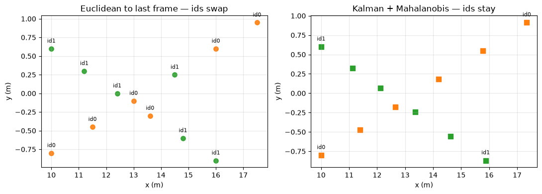
Two cars drive forward with noisy detections. On the right, a Kalman tracker with Mahalanobis matching should keep id 0 on the faster car and id 1 on the slower one. On the left, the same detections matched by Euclidean distance to stale positions should trade ids when the cars draw close.
You do not need the filter equations yet. This picture is where the notebook lands.
Predict: ids on the left panel will jump mid-run. The right panel keeps one color per car.
def crossing_detections(n_frames=6):
    dets = []
    for k in range(n_frames):
        dets.append(
            np.array(
                [
                    [10.0 + 1.5 * k, -0.8 + 0.35 * k],
                    [10.0 + 1.2 * k, 0.6 - 0.3 * k],
                ],
                dtype=np.float64,
            )
        )
    return dets


def naive_euclidean_track(detections_over_time):
    prev = None
    ids_for_det = []
    for dets in detections_over_time:
        dets = np.asarray(dets, dtype=np.float64)
        if prev is None:
            prev = dets.copy()
            ids_for_det.append([0, 1])
            continue
        cost = np.linalg.norm(prev[:, None, :] - dets[None, :, :], axis=2)
        row, col = linear_sum_assignment(cost)
        assign = [-1, -1]
        for r, c in zip(row, col):
            assign[c] = int(r)
        ids_for_det.append(assign)
        prev = dets.copy()
    return ids_for_det


cross_dets = crossing_detections()
naive_ids = naive_euclidean_track(cross_dets)
print("naive det ids per frame (det lane A, det lane B):")
for k, pair in enumerate(naive_ids):
    print(f"  frame {k}: {pair}")

KalmanBoxTracker.count = 0
mot = MultiObjectTracker(max_age=3, min_hits=1, distance_threshold=4.0)
kalman_by_frame = []
for dets in cross_dets:
    kalman_by_frame.append(mot.update(dets))

fig, axes = plt.subplots(1, 2, figsize=(11, 4))
colors = ["C1", "C2"]
ax = axes[0]
for fi, dets in enumerate(cross_dets):
    for dj in range(2):
        tid = naive_ids[fi][dj]
        ax.scatter(dets[dj, 0], dets[dj, 1], c=colors[tid], s=45, alpha=0.9)
        ax.text(dets[dj, 0], dets[dj, 1] + 0.08, f"id{tid}", fontsize=8, ha="center")
ax.set_title("Euclidean to last frame — ids swap")
ax.set_xlabel("x (m)")
ax.set_ylabel("y (m)")
ax.grid(True, alpha=0.3)

ax = axes[1]
for fi, frame in enumerate(kalman_by_frame):
    for tid, pos, vel in frame:
        c = colors[tid]
        ax.scatter(pos[0], pos[1], c=c, marker="s", s=45)
        if fi in (0, len(kalman_by_frame) - 1):
            ax.text(pos[0], pos[1] + 0.08, f"id{tid}", fontsize=8, ha="center")
ax.set_title("Kalman + Mahalanobis — ids stay")
ax.set_xlabel("x (m)")
ax.set_ylabel("y (m)")
ax.grid(True, alpha=0.3)
plt.tight_layout()
plt.show()

# Highway demo numbers (same seed as before) for recap alignment
KalmanBoxTracker.count = 0
np.random.seed(0)
ego = VectorLane("ego_centerline", [0.0, 0.02, 0.0005, 0.0])
tracker = MultiObjectTracker(max_age=3, min_hits=2, distance_threshold=4.0)
dt = 0.1
kalman_hw = []
for step in range(6):
    t = step * dt
    true_ax = 15.0 + 12.0 * t
    true_ay = ego.lateral_offset(true_ax)
    true_bx = 10.0 + 16.0 * t
    true_by = -3.5
    noisy = np.array(
        [
            [true_ax, true_ay] + np.random.normal(0, 0.15, size=2),
            [true_bx, true_by] + np.random.normal(0, 0.15, size=2),
        ]
    )
    kalman_hw.append(tracker.update(noisy))

bits0 = kalman_hw[0]
bits5 = kalman_hw[-1]
for label, frame in [("highway first", bits0), ("highway last", bits5)]:
    parts = [f"ID {tid}: ({pos[0]:.1f}, {pos[1]:.1f}) vx={vel[0]:.1f}" for tid, pos, vel in frame]
    print(label, "; ".join(parts))
naive det ids per frame (det lane A, det lane B):
  frame 0: [0, 1]
  frame 1: [0, 1]
  frame 2: [0, 1]
  frame 3: [1, 0]
  frame 4: [0, 1]
  frame 5: [0, 1]
highway first ID 0: (15.3, 0.5) vx=0.0; ID 1: (10.1, -3.2) vx=0.0
highway last ID 0: (20.6, 0.7) vx=8.7; ID 1: (17.9, -3.6) vx=13.2
On the left, frame 3 assigns [1, 0] instead of [0, 1]: the colors trade while the paths cross. A planner would think each car teleported into the other's lane.
On the right, ids stay on the same diagonal motion through the crossing. The highway run in that cell uses noisy detections like a real sensor: highway first ID 0: (15.3, 0.5) vx=0.0; ID 1: (10.1, -3.2) vx=0.0 and highway last ID 0: (20.6, 0.7) vx=8.7; ID 1: (17.9, -3.6) vx=13.2. That is the destination this notebook builds toward.
2. Detections flicker
One car, straight line. The lane center stays at y = 0, but the detector wiggles.
Predict: measured y will bounce even though the true path is flat.
np.random.seed(1)
true_pts, det_pts = [], []
print("frame true_x true_y det_x det_y")
for k in range(5):
    true_x = 20.0 + 10.0 * k * 0.1
    true_y = 0.0
    det = np.array([true_x, true_y]) + np.random.normal(0, 0.35, size=2)
    true_pts.append([true_x, true_y])
    det_pts.append(det)
    print(f"{k} {true_x:.1f} {true_y:.1f} {det[0]:.3f} {det[1]:.3f}")

true_pts = np.array(true_pts)
det_pts = np.array(det_pts)
plt.figure(figsize=(8, 3))
plt.scatter(true_pts[:, 0], true_pts[:, 1], c="k", marker="x", label="true")
plt.scatter(det_pts[:, 0], det_pts[:, 1], c="C1", label="detections")
plt.xlabel("x (m)")
plt.ylabel("y (m)")
plt.legend()
plt.title("True path vs noisy detections")
plt.grid(True, alpha=0.3)
plt.show()
frame true_x true_y det_x det_y
0 20.0 0.0 20.569 -0.214
1 21.0 0.0 20.815 -0.376
2 22.0 0.0 22.303 -0.806
3 23.0 0.0 23.611 -0.266
4 24.0 0.0 24.112 -0.087
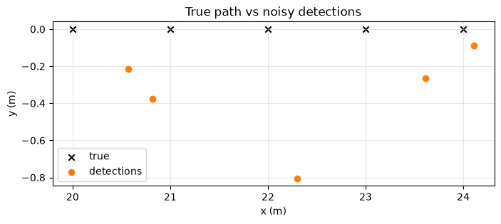
True y is 0.0 every frame, but measured y runs through -0.214, -0.376, -0.806, -0.266, and -0.087. Without a track id, each dot is a stranger. When the car hides, the next dot has no name attached.
3. Nearest neighbor swaps the IDs
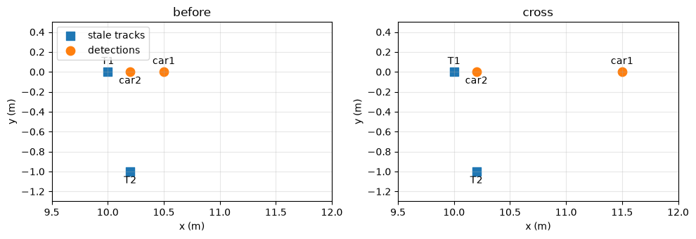
Two cars cross in x. Each track remembers last frame's detection. Euclidean distance picks the closest dot.
Predict: Track 1 will lock onto the wrong car when the dots overlap in x.
# Crossing paths: two frames where stale positions favor the wrong partner
frames = {
    "before": (np.array([10.0, 0.0]), np.array([10.2, -1.0]), np.array([10.5, 0.0]), np.array([10.2, 0.0])),
    "cross": (np.array([10.0, 0.0]), np.array([10.2, -1.0]), np.array([11.5, 0.0]), np.array([10.2, 0.0])),
}
fig, axes = plt.subplots(1, 2, figsize=(10, 3.5))
for ax, (title, (t1, t2, car1, car2)) in zip(axes, frames.items()):
    ax.scatter([t1[0], t2[0]], [t1[1], t2[1]], c="C0", s=80, marker="s", label="stale tracks")
    ax.scatter([car1[0], car2[0]], [car1[1], car2[1]], c="C1", s=80, label="detections")
    ax.annotate("T1", t1, textcoords="offset points", xytext=(0, 8), ha="center")
    ax.annotate("T2", t2, textcoords="offset points", xytext=(0, -12), ha="center")
    ax.annotate("car1", car1, textcoords="offset points", xytext=(0, 8), ha="center")
    ax.annotate("car2", car2, textcoords="offset points", xytext=(0, -12), ha="center")
    ax.set_title(title)
    ax.set_xlabel("x (m)")
    ax.set_ylabel("y (m)")
    ax.grid(True, alpha=0.3)
    ax.set_xlim(9.5, 12.0)
    ax.set_ylim(-1.3, 0.5)
axes[0].legend(loc="upper left")
plt.tight_layout()
plt.show()

t1 = np.array([10.0, 0.0])
t2 = np.array([10.2, -1.0])
car1 = np.array([11.5, 0.0])
car2 = np.array([10.2, 0.0])
d_t1_car1 = np.linalg.norm(t1 - car1)
d_t1_car2 = np.linalg.norm(t1 - car2)
print(f"Track 1 to car 1: {d_t1_car1:.2f} m")
print(f"Track 1 to car 2: {d_t1_car2:.2f} m")
print(f"ID SWAP: {d_t1_car2:.2f} < {d_t1_car1:.2f}")
cost = np.array([
    [np.linalg.norm(t1 - car1), np.linalg.norm(t1 - car2)],
    [np.linalg.norm(t2 - car1), np.linalg.norm(t2 - car2)],
])
print("euclidean cost")
print(np.round(cost, 2))
row, col = linear_sum_assignment(cost)
names_t = ["T1", "T2"]
names_d = ["car1", "car2"]
for r, c in zip(row, col):
    print(f"{names_t[r]} -> {names_d[c]}")
Track 1 to car 1: 1.50 m
Track 1 to car 2: 0.20 m
ID SWAP: 0.20 < 1.50
euclidean cost
[[1.5  0.2 ]
 [1.64 1.  ]]
T1 -> car2
T2 -> car1
Track 1 sits 0.20 m from car 2 but 1.50 m from car 1, so the matcher flips: T1 -> car2 and T2 -> car1. The crossing panel is the geometry behind section 1's color swap. For a car, that is a sudden lane-change hallucination on the wrong vehicle.
4. Kalman: guess forward, then nudge toward the dot
Kalman filtering is guess where it will be, then nudge the guess toward the measurement. First a one-number picture, then the repo's four-state tracker.
Predict: with loose prior variance P = 1 and tight sensor noise r = 0.09, a dot at z = 10.5 should pull the guess most of the way over and shrink uncertainty.
x, P, q, z, r = 10.0, 1.0, 0.0, 10.5, 0.09
P_pred = P + q
x_pred = x
K = P_pred / (P_pred + r)
x_post = x + K * (z - x)
P_post = (1.0 - K) * P_pred
print(f"P_pred = {P_pred:.4f}")
print(f"K = {K:.4f}")
print(f"x = {x_post:.4f}")
print(f"P = {P_post:.4f}")

fig, ax = plt.subplots(figsize=(6, 2.5))
ax.axvline(x, color="C0", lw=3, label="guess before")
ax.axvline(x_pred, color="C2", ls="--", lw=2, label="after predict")
ax.axvline(z, color="C1", marker="o", lw=0, markersize=8, label="camera z")
ax.axvline(x_post, color="C3", lw=3, label="after nudge")
ax.set_yticks([])
ax.set_xlim(9.7, 10.8)
ax.set_xlabel("x (m)")
ax.legend(loc="upper left")
ax.set_title("Scalar update: nudge toward z")
plt.tight_layout()
plt.show()
P_pred = 1.0000
K = 0.9174
x = 10.4587
P = 0.0826
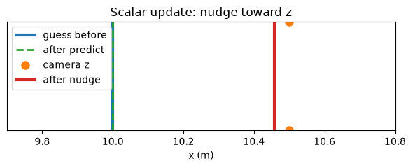
Gain is 0.9174, so the state lands at 10.4587, most of the way from 10.0 toward 10.5. Posterior variance 0.0826 is far below the prior 1.0000. For a car, that is trusting a fresh lidar dot without jerking the whole track.
Predict: KalmanBoxTracker rolls velocity forward on predict, then the same nudge on update should shrink the position covariance trace.
KalmanBoxTracker.count = 0
trk = KalmanBoxTracker(np.array([10.0, 0.0]), dt=0.1)
print(f"x shape {trk.x.shape}")
print(
    f"F {trk.F.shape} H {trk.H.shape} Q {trk.Q.shape} R {trk.R.shape} P {trk.P.shape}"
)
print(f"R diag {np.diag(trk.R)}")
trk.predict()
print(f"state after predict {np.round(trk.x, 6)}")
prior_trace = np.trace(trk.P[:2, :2])
print(f"prior position trace {prior_trace:.6f}")
trk.update(np.array([10.5, 0.0]))
post_trace = np.trace(trk.P[:2, :2])
print(f"posterior position trace {post_trace:.6f}")
print(f"state after update {np.round(trk.x, 6)}")
x shape (4,)
F (4, 4) H (2, 4) Q (4, 4) R (2, 2) P (4, 4)
R diag [0.09 0.09]
state after predict [10.  0.  0.  0.]
prior position trace 2.400000
posterior position trace 0.167442
state after update [10.465116  0.        0.387597  0.      ]
After predict the state is unchanged in position but velocity slots are ready to move. The position covariance trace drops from 2.400000 to 0.167442 once the [10.5, 0.0] measurement arrives. Same nudge story as the scalar line, now in x and y.
5. Mahalanobis distance knows which way you are uncertain
Same offset in meters can be normal or outrageous depending on variance. Mahalanobis stretches axes where the filter is tight.
Predict: innovation [0.3, 0.5] with S = diag(0.09, 0.25) will look farther in Mahalanobis than in raw meters.
S = np.diag([0.09, 0.25])
y = np.array([0.3, 0.5])
d2 = float(y @ np.linalg.inv(S) @ y)
print(f"d_M^2 = {d2:.1f}")
print(f"d_M = {np.sqrt(d2):.4f}")
print(f"euclidean = {np.linalg.norm(y):.4f}")
d_M^2 = 2.0
d_M = 1.4142
euclidean = 0.5831
Mahalanobis length is 1.4142 while Euclidean is only 0.5831. The first axis is tight in S, so a 0.3 m error there counts heavily. Association should use that yardstick, not plain meters.
Predict: after predict, Mahalanobis costs on the section 3 scene should put Track 1 on car 1 and Track 2 on car 2.
KalmanBoxTracker.count = 0
trk1 = KalmanBoxTracker(initial_pos=np.array([10.0, 0.0]))
trk1.x[2] = 15.0
trk1.x[3] = 0.0
trk2 = KalmanBoxTracker(initial_pos=np.array([10.2, -1.0]))
trk2.x[2] = 0.0
trk2.x[3] = 10.0
car1 = np.array([11.5, 0.0])
car2 = np.array([10.2, 0.0])
pred1 = trk1.predict()[:2]
pred2 = trk2.predict()[:2]
print(f"Track 1 predicted ({pred1[0]:.1f}, {pred1[1]:.1f})")
print(f"Track 2 predicted ({pred2[0]:.1f}, {pred2[1]:.1f})")
m11 = trk1.mahalanobis_distance(car1)
m12 = trk1.mahalanobis_distance(car2)
m21 = trk2.mahalanobis_distance(car1)
m22 = trk2.mahalanobis_distance(car2)
print(f"Mahalanobis T1->car1 {m11:.2f}")
print(f"Mahalanobis T1->car2 {m12:.2f}")
print(f"Mahalanobis T2->car1 {m21:.2f}")
print(f"Mahalanobis T2->car2 {m22:.2f}")
cost = np.array([[m11, m12], [m21, m22]])
row, col = linear_sum_assignment(cost)
for r, c in zip(row, col):
    print(f"{['T1','T2'][r]} -> {['car1','car2'][c]}  cost {cost[r, c]:.2f}")
Track 1 predicted (11.5, 0.0)
Track 2 predicted (10.2, 0.0)
Mahalanobis T1->car1 0.00
Mahalanobis T1->car2 1.14
Mahalanobis T2->car1 1.14
Mahalanobis T2->car2 0.00
T1 -> car1  cost 0.00
T2 -> car2  cost 0.00
Predictions sit at (11.5, 0.0) and (10.2, 0.0). On-diagonal Mahalanobis costs are 0.00 and off-diagonal are 1.14, so the assignment is T1 -> car1 and T2 -> car2. That is the fix behind the stable colors in section 1.
6. Coast when the camera blinks
Coasting is keep rolling when the camera blinks: predict with no new dot.
Predict: one empty frame after a speed seed should advance the same id with no measurement nudge.
KalmanBoxTracker.count = 0
mot = MultiObjectTracker(max_age=3, min_hits=2, distance_threshold=4.0)
seen = mot.update(np.array([[10.0, 0.0]]))
mot.trackers[0].x[2] = 12.0
mot.trackers[0].x[3] = 0.0
missed = mot.update(np.empty((0, 2)))
tid, pos, vel = missed[0]
print(f"seen id={seen[0][0]}")
print(f"coast id={tid} x={pos[0]:.1f} y={pos[1]:.1f} vx={vel[0]:.1f}")
print(f"time_since_update={mot.trackers[0].time_since_update}")
seen id=0
coast id=0 x=11.2 y=0.0 vx=12.0
time_since_update=1
The track keeps id 0, moves to x=11.2 with vx=12.0, and time_since_update=1 while no dot arrived. Behind a truck, the planner still has a place to aim until the detector returns.
7. Vector lanes (short)
Lanes live in the same x–y space as tracks. VectorLane turns a cubic polynomial into offset, heading, and curvature along forward distance.
Predict: a straight offset 2.0 m stays flat; a small quadratic coefficient bends lateral offset at large x.
straight = VectorLane("straight", [2.0, 0.0, 0.0, 0.0])
curved = VectorLane("curved", [0.0, 0.0, 0.001, 0.0])
ego = VectorLane("ego_centerline", [0.0, 0.02, 0.0005, 0.0])
for name, lane, x in [
    ("straight", straight, 15.0),
    ("curved", curved, 10.0),
    ("ego", ego, 30.0),
]:
    print(
        f"{name} x={x:.1f} offset={lane.lateral_offset(x):.2f} "
        f"heading={lane.heading_tangent(x):.4f} curvature={lane.curvature(x):.4f}"
    )
straight x=15.0 offset=2.00 heading=0.0000 curvature=0.0000
curved x=10.0 offset=0.10 heading=0.0200 curvature=0.0020
ego x=30.0 offset=1.05 heading=0.0500 curvature=0.0010
Straight lane offset is 2.00 with heading 0.0000. The curved lane hits offset 0.10 with positive curvature. Ego centerline offset at 30.0 m is 1.05, the same lane used in section 1 for car A.
proc = subprocess.run(
    [sys.executable, "-m", "pytest", "modules/05_vector_space", "-q"],
    capture_output=True,
    text=True,
    cwd=str(REPO),
)
print(proc.stdout.strip())
print("returncode", proc.returncode)
assert proc.returncode == 0
...                                                                      [100%]
3 passed in 0.27s
returncode 0
Module tests report 3 passed. The numbers above match what pytest checks in the repo tracker.
8. Exercises
Exercise — scalar update. Return Kalman gain, posterior mean, and posterior variance for a constant-position scalar with process noise q. Leave the TODO as it is to use the reference implementation.
Predict: your function should match section 4 numbers for (x, P, z, q, r) = (10.0, 1.0, 10.5, 0.0, 0.09).
def scalar_update_student(x, P, z, q, r):
    # TODO: constant-position Kalman update; return K, x_post, P_post
    raise NotImplementedError

def reference_scalar_update(x, P, z, q, r):
    P_pred = P + q
    K = P_pred / (P_pred + r)
    x_post = x + K * (z - x)
    P_post = (1.0 - K) * P_pred
    return K, x_post, P_post

def get_scalar_update():
    try:
        scalar_update_student(10.0, 1.0, 10.5, 0.0, 0.09)
    except NotImplementedError:
        print("Using reference scalar_update (TODO not implemented)")
        return reference_scalar_update
    return scalar_update_student

fn = get_scalar_update()
K, x_post, P_post = fn(10.0, 1.0, 10.5, 0.0, 0.09)
assert np.isclose(K, 0.9174, atol=1e-4)
assert np.isclose(x_post, 10.4587, atol=1e-4)
assert np.isclose(P_post, 0.0826, atol=1e-4)
print(f"K = {K:.4f}")
print(f"x = {x_post:.4f}")
print(f"P = {P_post:.4f}")
print("✅ correct: scalar update")
Using reference scalar_update (TODO not implemented)
K = 0.9174
x = 10.4587
P = 0.0826
✅ correct: scalar update
Gain 0.9174, state 10.4587, variance 0.0826 match section 4. The reference implementation ran because the TODO still raises.
Solution
def scalar_update_student(x, P, z, q, r):
    P_pred = P + q
    K = P_pred / (P_pred + r)
    x_post = x + K * (z - x)
    P_post = (1.0 - K) * P_pred
    return K, x_post, P_post
Exercise — Mahalanobis distance. Return sqrt(y^T S^{-1} y) for innovation y and covariance S.
Predict: on y=[0.3, 0.5] and S=diag(0.09, 0.25) you should match section 5.
def mahalanobis_student(y, S):
    # TODO: return sqrt(y^T S^{-1} y)
    raise NotImplementedError

def reference_mahalanobis(y, S):
    y = np.asarray(y, dtype=np.float64)
    S = np.asarray(S, dtype=np.float64)
    d2 = float(y @ np.linalg.inv(S) @ y)
    return float(np.sqrt(max(0.0, d2)))

def get_mahalanobis():
    try:
        mahalanobis_student(np.array([0.3, 0.5]), np.diag([0.09, 0.25]))
    except NotImplementedError:
        print("Using reference mahalanobis (TODO not implemented)")
        return reference_mahalanobis
    return mahalanobis_student

mfn = get_mahalanobis()
d_M = mfn(np.array([0.3, 0.5]), np.diag([0.09, 0.25]))
assert np.isclose(d_M, 1.4142, atol=1e-4)
print(f"d_M = {d_M:.4f}")
print("✅ correct: mahalanobis")
Using reference mahalanobis (TODO not implemented)
d_M = 1.4142
✅ correct: mahalanobis
Distance 1.4142 matches section 5. The reference implementation ran because the TODO still raises.
Solution
def mahalanobis_student(y, S):
    y = np.asarray(y, dtype=np.float64)
    S = np.asarray(S, dtype=np.float64)
    d2 = float(y @ np.linalg.inv(S) @ y)
    return float(np.sqrt(max(0.0, d2)))
9. Recap
- Noisy dots wiggle in
y(-0.214,-0.376,-0.806,-0.266,-0.087) while the lane center stays0.0. - Euclidean matching flipped ids (
0.20m vs1.50m) and assignedT1 -> car2; crossing frames swapped to[1, 0]at frame3. - Kalman nudge:
K = 0.9174,x = 10.4587,P = 0.0826; matrix trace fell from2.400000to0.167442. - Mahalanobis kept
T1 -> car1at cost0.00; coasting held id0atx=11.2withvx=12.0. - Highway demo ended at
vx=8.7andvx=13.2with stable ids; module tests:3 passed.