Week 4 · 4 hours

Closing the loop

The box you build: Controller: the steering law that turns your lane estimate into a wheel angle, every 0.05 s

What you will be able to do

  • Explain why a closed-loop controller corrects an error that an open-loop plan lets grow, and write a P steering law with the right signs, the 0.5 rad clip and a straight wheel when the estimate is not valid

    Proof Your p_steer passes the Exercise A check in the lab, and the quiz questions on open loop and on signs

  • Predict what too little and too much gain do to the car, and explain why the wheel's 1 rad/s limit caps the useful gain

    Proof Practice problem 1 and the tuning and break-it sections of the lab, and the quiz questions on the two gains and on k_off = 6

  • Build a car that runs your own perception and your own controller, and complete gentle with it

    Proof Your my_car passes the Exercise B check in the lab

  • Compute the offset a P-steered car carries in a steady bend, and explain why the car with the two-point box leaves curvy

    Proof Practice problems 2 and 3 and the inside-the-bend section of the lab, and the quiz questions on bends and on curvy

Before this: Week 3 · Your first perception box

Warm-up review

Nothing is due today. Pass a week's quiz and its questions come back here at growing intervals.

Lecture

Open loop and closed loop

Your car now sees through your perception box. This unit opens the last box, the controller: every 0.05 s it receives your LaneEstimate and returns a steering angle.

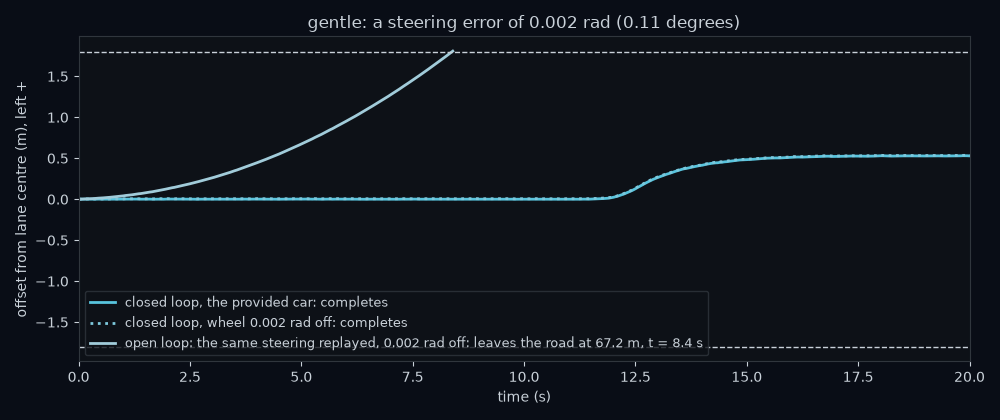
Record every steering angle the provided car used on its lap of gentle, then replay the recording without looking at the camera. Replayed exactly, it gives the same lap. Now set the wheel 0.002 rad (0.11 degrees) off. The replayed car leaves the road after 67.2 m, 8.4 s in, still on the first straight. The provided car, with the same 0.002 rad error, completes the lap with a mean |lateral error| of 0.381 m instead of 0.376 m.

How we got 0.11 degrees

Angles in the simulator are in radians: a full turn is 2π2\pi radians, and also 360°360°. So one radian is 360°/2π=180°/π=57.30°360° / 2\pi = 180° / \pi = 57.30°. Then

0.002 rad×57.30 degrees per radian=0.115°≈0.11°0.002 \text{ rad} \times 57.30 \text{ degrees per radian} = 0.115° \approx 0.11°
Offset against time on gentle. The provided car and the provided car with the wheel 0.002 rad off overlap and complete; the replayed steering drifts steadily left and leaves the road at 8.4 s.
Figure 1. Offset against time on gentle. The provided car and the provided car with the wheel 0.002 rad off overlap and complete; the replayed steering drifts steadily left and leaves the road at 8.4 s.

The replay is open loop: its commands were fixed in advance, so nothing notices the error and it adds up. The provided car is closed loop: each command is computed from the latest measurement, so an error is corrected as soon as it shows. Åström and Murray define it:

"The term feedback refers to a situation in which two (or more) dynamical systems are connected together such that each system influences the other" (§1.1)

Here the two systems are the car, turning a steering angle into a new position, and the controller, turning the camera's view of that position into the next steering angle.

The P controller

The 2006 paper on Stanford's robot car Stanley puts it in one line: "The larger this error, the stronger the steering response toward the trajectory." (Thrun et al., p. 684). The simplest law with that property is proportional control:

u=kp (r−y)=kp eu = k_p\,(r - y) = k_p\,e

(Åström & Murray, Eq. 1.3). Here uu is the controller's output, rr the reference (the value you want), yy the measured value, e=r−ye = r - y the control error and kpk_p the gain, how hard to push per unit of error.

For your car, uu is the steering angle δ\delta (radians, left positive), the reference is offset 0 and the measurement is the offset eoffe_{\text{off}}. So r−y=−eoffr - y = -e_{\text{off}} and

δ=−koff eoff\delta = -k_{\text{off}}\, e_{\text{off}}

with koffk_{\text{off}} in radians of wheel per metre. The minus sign is the whole point: 0.4 m left of centre with koff=0.35k_{\text{off}} = 0.35 gives δ=−0.14\delta = -0.14 rad, steering right, towards the centre. Steering against the error is negative feedback; drop the minus sign and you get unit 0.1.3's positive feedback.

Two guards complete the law:

  • Clip the result to ±0.5 rad, the furthest the simulator's wheel turns, with np.clip.
  • If est.valid is False, return 0.0: hold the wheel straight rather than steer on NaNs.

Two errors, two gains

A car on lane centre but pointing 0.05 rad left is fine now, not in a second: at 8 m/s it moves 8sin⁡0.05=0.408 \sin 0.05 = 0.40 m sideways every second. A heading error is an offset in the making, so the controller uses both errors:

δ=−(koff eoff+khead ψ),clipped to ±0.5\delta = -\left(k_{\text{off}}\, e_{\text{off}} + k_{\text{head}}\, \psi\right), \quad \text{clipped to } \pm 0.5

where ψ\psi is the heading in radians, left positive, and kheadk_{\text{head}} has no units. The provided car uses koff=0.35k_{\text{off}} = 0.35 and khead=2.7k_{\text{head}} = 2.7.

How we got 0.40 m sideways per second

The car moves 8 m every second along the direction it points. If that direction is ψ=0.05\psi = 0.05 rad away from the road's direction, only part of the 8 m is along the road. The rest is sideways, and trigonometry gives the sideways part of a distance as the distance times sin⁡\sin of the angle:

8×sin⁡0.05=8×0.04998=0.3998≈0.40 m8 \times \sin 0.05 = 8 \times 0.04998 = 0.3998 \approx 0.40 \text{ m}

(The sin⁡\sin must be taken with the angle in radians, as here.)

Worked example. The car is 0.4 m left of centre and pointing 0.05 rad left:

δ=−(0.35×0.4+2.7×0.05)=−(0.14+0.135)=−0.275 rad\delta = -(0.35 \times 0.4 + 2.7 \times 0.05) = -(0.14 + 0.135) = -0.275 \text{ rad}

Firmly right. Same offset, but pointing 0.05 rad right, back towards the centre: δ=−(0.14−0.135)=−0.005\delta = -(0.14 - 0.135) = -0.005 rad, almost straight. The car is already coming back, so the controller eases off. Without the heading term it would steer right all the way to the centre, arrive pointing across the lane and swing past.

The lab pushes the car 1.10 m left, then hands over to the P law with koff=0.35k_{\text{off}} = 0.35. With khead=0k_{\text{head}} = 0 the car swings 0.30 m past the centre. With khead=1k_{\text{head}} = 1 it settles within 5 cm in 1.15 s, never a millimetre past. With khead=2.7k_{\text{head}} = 2.7 it creeps back and takes 3.10 s. The heading gain is a brake on the swing: too little overshoots, too much is sluggish.

Tuning the gains

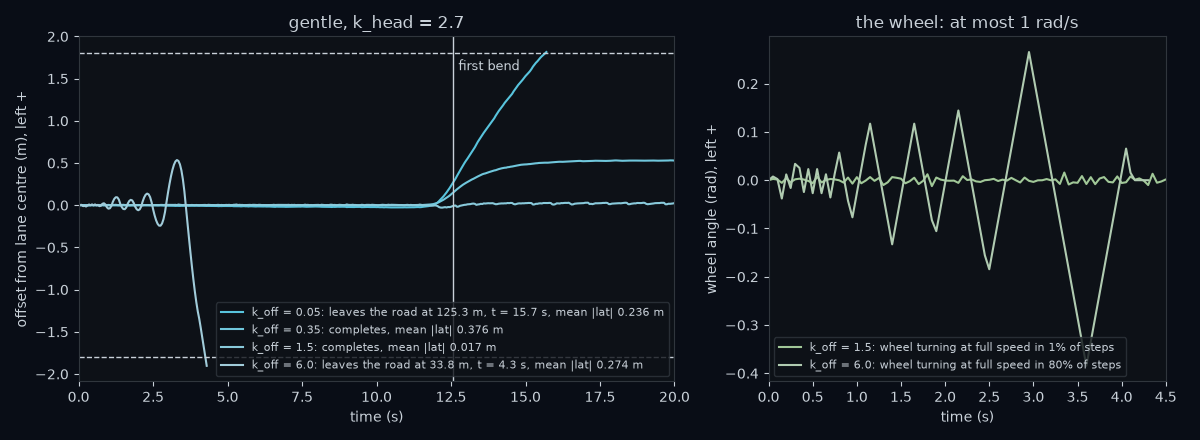
Keep khead=2.7k_{\text{head}} = 2.7 and sweep koffk_{\text{off}} on gentle:

Left: offset against time for four values of k_off; 0.05 drifts off at the first bend, 6 swings ever wider and leaves on the straight. Right: the wheel angle, smooth for 1.5, zigzagging at full speed for 6.
Figure 2. Left: offset against time for four values of k_off; 0.05 drifts off at the first bend, 6 swings ever wider and leaves on the straight. Right: the wheel angle, smooth for 1.5, zigzagging at full speed for 6.
  • koff=0.05k_{\text{off}} = 0.05: offsets go uncorrected for seconds; at the first bend the car drifts inside and leaves the road at 125.3 m.
  • 0.350.35, the provided value: completes, mean |lateral error| 0.376 m.
  • 1.51.5: completes, 0.017 m.
  • 3.03.0 (in the lab): completes, 0.042 m.
  • 6.06.0: leaves the road after 33.8 m, 4.3 s in, still on the first straight.

The tempting conclusion is "more gain, tighter tracking". It holds from 0.05 to 1.5, then fails: 3.0 is worse than 1.5, and 6.0 crashes. The reason is the wheel, which turns at most 1 rad/s. With koff=6k_{\text{off}} = 6, a 5 cm offset asks for 0.3 rad of wheel, which takes 0.3 s to reach, 2.4 m of travel at 8 m/s. By then the car has crossed the centre and the controller wants the opposite. The right panel shows it: at koff=6k_{\text{off}} = 6 the wheel turns at full speed in 80% of steps, always late, each swing wider than the last. There is a best range of gains, and the car's limits set its top.

How we got 0.3 rad, 0.3 s and 2.4 m

Three small steps, each feeding the next.

  1. Wheel angle asked for. With only the offset term, δ=koff×eoff\delta = k_{\text{off}} \times e_{\text{off}} in size. A 5 cm offset is 0.050.05 m, so δ=6×0.05=0.3\delta = 6 \times 0.05 = 0.3 rad.
  2. Time to turn the wheel there. The wheel turns at most 1 radian per second, so 0.3 rad takes 0.3/1=0.30.3 / 1 = 0.3 s. In the simulator's 0.05 s steps that is 6 steps.
  3. Distance driven meanwhile. At 8 m/s, 8×0.3=2.48 \times 0.3 = 2.4 m.

Why curves need error

To follow a circle of radius RR, a car with wheelbase L=2.7L = 2.7 m (front axle to rear axle) holds its wheel at about

δ≈arctan⁡LR\delta \approx \arctan\frac{L}{R}

because the car turns about the point where lines drawn square to its front and rear wheels meet. On gentle's bends your lane has radius 81.8 m (80 m plus 1.8 m: your lane is on the outside), so δ=arctan⁡(2.7/81.8)=0.0330\delta = \arctan(2.7 / 81.8) = 0.0330 rad.

How we got δ=0.0330\delta = 0.0330 rad

First the lane's radius. The road's centre line (the yellow line) bends left with radius 80 m. Your lane's centre is 1.8 m to the right of it, which on a left bend is the outside, so its circle is bigger: 80+1.8=81.880 + 1.8 = 81.8 m.

Then the ratio of wheelbase to radius: L/R=2.7/81.8=0.03301L / R = 2.7 / 81.8 = 0.03301. The arctan⁡\arctan turns this ratio into an angle in radians:

arctan⁡(0.03301)=0.03300≈0.0330 rad\arctan(0.03301) = 0.03300 \approx 0.0330 \text{ rad}

For a ratio this small the angle and the ratio are almost the same number.

A P law turns the wheel only when there is error. With both errors zero it says δ=0\delta = 0, and the car runs straight off the circle. So in a steady bend the car must carry errors that add up to the right δ\delta.

Which errors? The car's position is measured at its front axle, which travels where the front wheels point: the car's heading plus δ\delta. For the front axle to run along the lane, the front wheels point along the lane, so the body points δ\delta to the outside: ψ=−δ\psi = -\delta on a left bend. The heading term then gives −kheadψ=2.7 δ-k_{\text{head}}\psi = 2.7,\delta, 2.7 times what is needed. The offset term must take back the extra 1.7 δ1.7,\delta: koff eoff=(khead−1) δk_{\text{off}}, e_{\text{off}} = (k_{\text{head}} - 1),\delta, so

eoff=(khead−1) δkoffe_{\text{off}} = \frac{(k_{\text{head}} - 1)\,\delta}{k_{\text{off}}}

Worked example. On gentle: 1.7×0.0330/0.35=0.1601.7 \times 0.0330 / 0.35 = 0.160 m, to the left, the inside of the bend. Given perfect lane values instead of your box's, the car settles at 0.162 m.
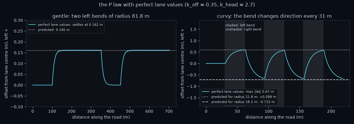
Left: with perfect lane values, the offset on gentle rises in each bend to the predicted 0.160 m. Right: on curvy the offset swings towards +0.60 m in left bends and -0.72 m in right bends.
Figure 3. Left: with perfect lane values, the offset on gentle rises in each bend to the predicted 0.160 m. Right: on curvy the offset swings towards +0.60 m in left bends and -0.72 m in right bends.

On curvy the bends have radius 20 m, so your lane's radius is 21.8 m on left bends and 18.2 m on right bends: δ=0.123\delta = 0.123 and 0.1470.147 rad, predicting 0.599 m and −0.715 m. Each bend is only 31 m long, so the offset is still moving when the next one begins; with perfect lane values the car stays within 0.67 m and completes curvy.

How we got 0.123, 0.147, 0.599 and −0.715

Do the gentle recipe twice, once for each side: first the lane's radius RR, then the wheel angle δ=arctan⁡(L/R)\delta = \arctan(L/R) with L=2.7L = 2.7 m, then the offset eoff=(khead−1) δ/koff=1.7 δ/0.35e_{\text{off}} = (k_{\text{head}} - 1),\delta / k_{\text{off}} = 1.7,\delta / 0.35.

  • Left bends. The lane is on the outside: R=20+1.8=21.8R = 20 + 1.8 = 21.8 m. δ=arctan⁡(2.7/21.8)=arctan⁡(0.12385)=0.12323≈0.123\delta = \arctan(2.7 / 21.8) = \arctan(0.12385) = 0.12323 \approx 0.123 rad. Offset =1.7×0.12323/0.35=+0.599= 1.7 \times 0.12323 / 0.35 = +0.599 m, positive because the car sits to the left, the inside.
  • Right bends. The lane is on the inside: R=20−1.8=18.2R = 20 - 1.8 = 18.2 m. δ=arctan⁡(2.7/18.2)=arctan⁡(0.14835)=0.14728≈0.147\delta = \arctan(2.7 / 18.2) = \arctan(0.14835) = 0.14728 \approx 0.147 rad. The bend is mirrored, so the offset is negative: −1.7×0.14728/0.35=−0.715-1.7 \times 0.14728 / 0.35 = -0.715 m.

The offsets come from the unrounded δ\delta. Starting from the rounded 0.123 and 0.147 would give 0.597 and 0.714 instead.

Åström and Murray name this: "proportional control has the drawback that the process variable often deviates from its reference value" (§1.6). Here the deviation grows as the bend tightens, because δ≈L/R\delta \approx L/R.

Set khead=1k_{\text{head}} = 1 and the offset vanishes. Stanley's law, Eq. 7, is δ(t)=ψ(t)+arctan⁡k x(t)u(t)\delta(t) = \psi(t) + \arctan\frac{k,x(t)}{u(t)}, where "The angle ψ […] describes the orientation of the nearest path segment, measured relative to the vehicle's own orientation" (p. 684): minus your heading, with gain exactly 1. Module 1.3 derives it.

Why your car leaves curvy

With perfect lane values the P law gets round curvy. The provided car does not: it leaves the road at 48.3 m, 6.1 s in, off the inside of the first left bend. Yours will too, if your box works like it.
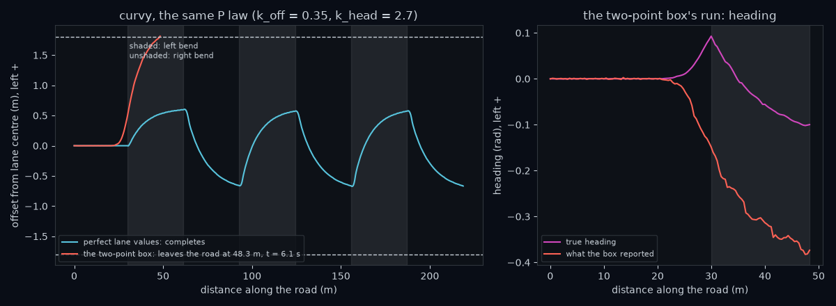
Left: on curvy, perfect lane values stay within 0.67 m; the two-point box drifts left before the first bend and leaves at 48.3 m. Right: the box's heading lies far right of the true heading.
Figure 4. Left: on curvy, perfect lane values stay within 0.67 m; the two-point box drifts left before the first bend and leaves at 48.3 m. Right: the box's heading lies far right of the true heading.

The cause is unit 0.1.3's chord bias: on a left bend the box says "left of centre, pointing right" even when the car is centred, and the controller multiplies the heading by 2.7. It starts early: the far band sees 5.6 to 11.5 m ahead, so at 30.3 m, just after the bend begins at 30 m, the car is already 0.56 m left.

Worked example. At 44.3 m the car is truly 1.701 m left, heading −0.0848 rad; the box reports 2.321 m and −0.3416 rad.

  • On the true values: −(0.35×1.701+2.7×(−0.0848))=−(0.595−0.229)=−0.366-(0.35 \times 1.701 + 2.7 \times (-0.0848)) = -(0.595 - 0.229) = -0.366 rad, hard right, back to the centre.
  • On the box's values: −(0.35×2.321+2.7×(−0.3416))=−(0.812−0.922)=+0.110-(0.35 \times 2.321 + 2.7 \times (-0.3416)) = -(0.812 - 0.922) = +0.110 rad, left, deeper inside.

A heading error of 0.3416−0.0848=0.2570.3416 - 0.0848 = 0.257 rad times 2.7 is 0.69 rad of phantom left steering, outweighing everything else.

Retuning can hide this: koff=1.5k_{\text{off}} = 1.5, or khead=1k_{\text{head}} = 1, gets round curvy (mean errors 0.085 and 0.131 m), but the bias remains. The real fixes are perception that fits the curve (module 1.5) and a controller that looks ahead along the road (module 1.3).

Closing the loop

Your last step is my_car = Car(perception=estimate_lane, controller=my_controller), where my_controller(est, obs) returns p_steer(est, K_OFF, K_HEAD). A controller that returns a number is a steering angle; the Car pairs it with the provided speed controller, which holds 8 m/s (module 1.2).

Check 0.1.4.b requires a Car running neither provided box to complete gentle with a mean |lateral error| below 0.5 m. Then it drives curvy, ungraded, so you see what your own car does there. Every box is now yours.

A 1988 car that learned to steer

Your car has hand-written perception and control. In 1988, Dean Pomerleau replaced both with one network: ALVINN, "a 3-layer back-propagation network designed for the task of road following" (p. 305).

  • Inputs: a 30x32 video retina fed the blue colour band, an 8x32 laser range-finder retina and one feedback unit: 1217 inputs, into 29 hidden units.
  • Outputs: 45 direction units, from sharp left to sharp right, the middle one "travel straight ahead" (p. 306). Its training target is the curvature "which would bring the vehicle to the road center 7 meters ahead of its current position" (p. 306): it aims at a point ahead, not at the error at the car.
  • Training: 1200 simulated road snapshots.
  • Result: it drove the NAVLAB van "at a speed of 1/2 meter per second along a 400 meter path through a wooded area" (pp. 308–309). CMU's traditional system, on the faster Warp computer, managed 1 m/s.
  • Limit: at a fork it could output two directions, and "The result is often an oscillation" (p. 312).
How we got 1217 inputs

Each retina is a grid of units, one per picture cell, so its size is rows times columns: the video retina has 30×32=96030 \times 32 = 960 units and the range-finder retina has 8×32=2568 \times 32 = 256. Add the one feedback unit:

960+256+1=1217960 + 256 + 1 = 1217

It is this module's paper.

Go deeper

  • Åström & Murray, "Feedback Systems" (2nd ed.), §1.1 "What Is Feedback?" and §1.6 "Simple Forms of Feedback": proportional control and its offset.
  • Thrun et al., "Stanley: The Robot that Won the DARPA Grand Challenge" (2006), §9.2 "Steering Control", Eq. 7 and Figure 24 (p. 684).
  • Pomerleau, "ALVINN: An Autonomous Land Vehicle in a Neural Network" (1988): start with Figure 1 and "Network Architecture".

Go deeper

Paper: ALVINN: An Autonomous Land Vehicle in a Neural Network (Pomerleau, NIPS 1988)

While you read, answer:

  • How big is the picture ALVINN "sees", and how many numbers is that?
  • Which colour channel does the video retina use, and why?
  • What does each output unit stand for, and what does the middle one mean?
  • Why didn't Pomerleau train on real road photos, and what did he use instead?
  • What did the real vehicle actually do, and how did that compare with the traditional method?
  • Name one thing the author says ALVINN could not yet do well.

Lab

Write the box in Colab and run its checks. Come back here for the quiz.

Open lab in Colab

Checkpoint quiz

1.

The provided car's steering on gentle is recorded and replayed without the camera, with the wheel 0.002 rad off. The replay leaves the road on the first straight; the provided car with the same error completes the lap. Why?

2.

The car is 0.3 m right of lane centre, pointing along the lane. A teammate's controller returns −0.105-0.105 rad. What is wrong?

3.

Your p_steer gets LaneEstimate(offset_m=-0.5, heading_rad=0.1, valid=True) with k_off = 0.4 and k_head = 1.0. What does it return, in radians?

4.

On gentle, with k_head = 2.7, raising k_off from 0.35 to 1.5 cuts the mean |lateral error| from 0.376 m to 0.017 m. What do you expect at k_off = 6?

5.

A car with wheelbase L=2.7L = 2.7 m follows a circle of radius 40 m. About what wheel angle, in radians, does it hold?

6.

With perfect lane values and k_off = 0.35, which k_head makes the settled offset in a long steady bend exactly zero?

7.

With perfect lane values, the P law (0.35, 2.7) completes curvy. Your car, with the same law and the two-point box, leaves the road at 48.3 m. Why?

8.

What did ALVINN's network output?

Teach it back

Explain this week as if to a friend who has never seen it. Then paste it, with the prompt below, into any AI tutor and ask it to find the gaps.

Show the tutor prompt
You are a Socratic tutor for unit 0.1.4 "Closing the loop" of a self-driving car course. I am a programmer with rusty maths and no machine-learning background. I have just read a lecture and done a lab on steering a car from its lane estimate with feedback.

What the unit taught (use these facts exactly):
- The simulator is a flat-world teaching simulator. Every 0.05 s the controller receives the lane estimate (offset in metres and heading in radians, left positive) and returns a steering angle in radians, left positive. The car drives at 8 m/s, its wheelbase is L = 2.7 m, the wheel turns at most 0.5 rad either way and at most 1 rad/s.
- Open loop replays fixed commands and never measures the result: the provided car's steering replayed with the wheel 0.002 rad off leaves gentle after 67.2 m. Closed loop computes each command from the latest measurement: the provided car with the same error completes, mean |lateral error| 0.381 m instead of 0.376 m.
- The P law: delta = -(k_off * offset + k_head * heading), clipped to plus or minus 0.5 rad, and 0.0 when the estimate is not valid. The minus sign steers against the error (negative feedback). The provided gains are k_off = 0.35 and k_head = 2.7. Example: 0.4 m left, pointing 0.05 rad left gives -0.275 rad; pointing 0.05 rad right instead gives -0.005 rad.
- The heading term acts as a brake on the swing: pushed 1.10 m left with k_off = 0.35, k_head = 0 overshoots the centre by 0.30 m, k_head = 1 settles in 1.15 s, k_head = 2.7 takes 3.10 s.
- Sweeping k_off on gentle with k_head = 2.7: 0.05 leaves the road at 125.3 m; 0.35 gives 0.376 m; 1.5 gives 0.017 m; 3.0 gives 0.042 m; 6.0 leaves after 33.8 m, because the wheel's 1 rad/s limit makes every correction late.
- Holding a circle of radius R needs delta about arctan(L / R). In a steady bend the body points delta to the outside (heading = -delta), so the P law settles at offset = (k_head - 1) * delta / k_off: 0.160 m on gentle's bends of radius 81.8 m. With k_head = 1 the offset is zero.
- With perfect lane values the P law completes curvy. With the two-point box it leaves curvy at 48.3 m: on a left bend the box reports a heading far to the right of the truth, and k_head = 2.7 turns that bias into steering left, deeper inside the bend.
- Misconception to probe: "more gain, tighter tracking". It holds only up to a point; past it the rate-limited wheel is always late and the car oscillates.

How to run the session:
1. Ask me ONE question at a time, then wait for my answer. Start by asking me why a tiny steering error crashes a replayed plan but not a car that steers from its measurements.
2. Never give me the answer. If I am wrong or vague, ask a smaller question, or give me numbers to work through by hand, so I find the mistake myself.
3. Within the first three questions, test the misconception: ask what I expect if k_off goes from 1.5 to 6, and why.
4. Ask at least one question where I compute a steering angle from an offset and heading you give me, one where I explain what the heading term does when the car is already heading back to the centre, and one where I compute the settled offset in a bend of a radius you give me.
5. Keep your turns short: two or three sentences, then the question.
6. After about five exchanges, stop. List what I explained well, and what I should revisit, naming these lecture sections: "Open loop and closed loop", "The P controller", "Two errors, two gains", "Tuning the gains", "Why curves need error", "Why your car leaves curvy", "Closing the loop", "A 1988 car that learned to steer".

Pilot log

0 logged

Saved in this browser. It tells the course author where this week is hard.

Confidence (1 = lost, 5 = could teach it)